Options Pricing Model

"Pricing Model for Ultra-Short Term Cryptocurrency Derivatives" By: Serge Bourenkov, July 29, 2023.

Abstract

This article addresses the complex problem of pricing ultra-short-term derivatives (30 to 90 minutes) in the cryptocurrency domain, particularly focusing on Ethereum (ETH/USD)-based instruments. Our research reveals that the distribution of price fluctuations in this market exhibits heavy tails. We have developed a mathematical model that accurately describes these unique distribution characteristics.

A key finding is that the widely used Black-Scholes model is not suitable for this context, prompting us to propose an alternative approach. Our methodology involves robust statistical models for predicting volatility, tailored to the nuances of cryptocurrency markets. This approach was rigorously tested on a substantial dataset of ETH/USD prices, demonstrating the model’s effectiveness and practical viability.

The results of this study have far-reaching implications for the pricing of derivatives in cryptocurrency markets, offering a significant advancement in understanding and managing the unique risks associated with these assets.

Introduction

Since Bitcoin’s inception, cryptocurrency markets have experienced substantial growth. By the end of 2022, the market peaked at a remarkable size, necessitating efficient trade facilitation. Over 200 centralized and decentralized exchanges have emerged, boasting substantial daily trading volumes. With the maturation of trading activities, an increasing number of exchanges are offering options trading, a crucial component of a developed market.

However, traditional options trading, with its complex terminology and limited opportunities, is often inaccessible to the majority of traders and poses potentially unlimited risks. To address these challenges, War of Coins has developed a new derivative instrument akin to options but simpler and more accessible. Traders only decide on the trade direction (put vs. call), with their risk capped at the purchase amount. These derivatives, offering profits up to 100 times the purchase amount, mature in under 90 minutes, aligning with traders’ preference for prompt results.

The system generates a ladder of price points that lists potential profits for multiple strike prices, ranging from equal to the purchase amount to 100 times. The best part is that traders don’t need to choose a specific price point like in traditional options trades. They just need to predict the price direction, with greater price movements in their favour resulting in larger profits.

Pricing short-term derivatives are notoriously challenging due to the non-normal distribution of short-term price fluctuations, characterized by "heavy" or "long" tails. This phenomenon, initially identified by Mandelbrot in 1963, suggested that financial instruments might follow Pareto-type or alpha-distributions. Subsequent research, such as that by Maslov et al. in 2001, further noted that short-term distribution tails follow a power law rather than an exponential one. Our analysis confirms this for Ethereum (ETH/USD) price fluctuations. We define price fluctuations as the fluctuation of absolute returns, i.e., the logarithm of relative price changes.

Our mathematical model closely matches historical data for 1-minute price fluctuations and, with minor adjustments, can describe fluctuations within the 30 to 90-minute range.

We acknowledge heteroscedasticity in our model, necessitating a method for predicting upcoming period volatility. To this end, we developed an approach based on robust statistics from multiple previous periods, diverging from traditional regression methods, fundamental factor analysis, or neural network-based approaches.

Traditional models like Black-Scholes, based on geometric random walk assumptions, are inadequate for power law distributions. We propose a novel pricing model using a price ladder for potential returns, ranging from 1 to 100 times the purchase value. This model, validated against 19 months of ETH/USD historical data, has shown consistent performance across different market conditions and maturity periods. The first 15 months of data were used for model evaluation and tuning, while the subsequent four months validated the model’s efficacy.

Analysis of historical ETH/USD price data at 1-minute intervals

The analysis was done on a 1-minute OHLC (open-high-low-close) ETH/USD price data obtained from the Coinbase cryptocurrency exchange. The data covers the period from Jan 1, 2022, to September 1, 2023. The period from January 1, 2022, to March 31, 2023 (15 months) has been used for the analysis and development of the pricing model. The remaining data from April 1, 2023, to September 1, 2023 (4 months) has been used for validation of model performance.

Fig. 1. gives the overview of the data in that period. For clarity, the chart shows only daily changes in the ETH/USD price. The second graph on the chart shows the value of the volatility predictor, smoothed by a 7-day moving average. The method for the prediction of volatility is explained in the corresponding section below.

Fig. 1. Overview of the data used in the analysis.

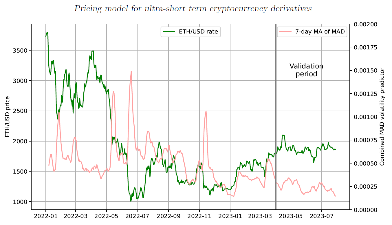
The data shows that during the period both the price and the volatility of the ETH changed in a wide range. There were periods of downward and upward trends as well as periods when the price was fairly stable.

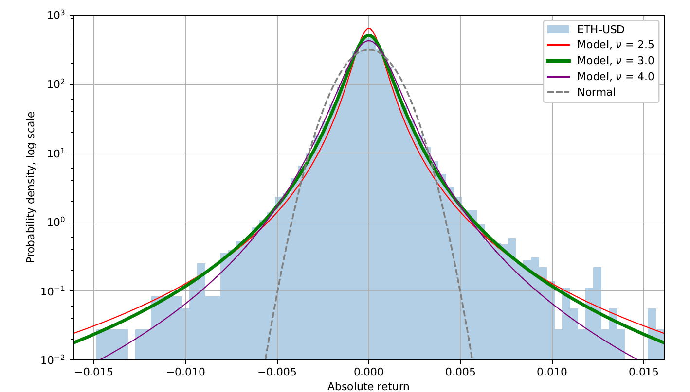
The chart in Fig. 2. shows the distribution of the price fluctuations in the 2 months from January 1, 2022, to March 1, 2022. Here and further in this article, we refer to changes in ”absolute return” as price fluctuations. Traditionally absolute return is defined as $log(p_1/p_0)$, where $p_0$ is the price of the previous time interval (minute, hour, day and so on). The black dotted line shows what normal distribution would have been like for the data with the same standard deviation. The observed distribution has characteristic “fat tails”, meaning that the probability density function (PDF) diminishes much slower than $exp (−x2)$.

This effect has been noticed by many researchers before. Benoit Mandelbrot's (1963) paper suggested that financial processes by their nature may not follow normal distribution law and suggested that Pareto-type distribution (or in a more general form alpha-distribution) may be better suited for that purpose. Other authors (Maslov et al, 2001) also concluded that in many cases such distribution has tails that follow power, rather than exponential, law.

We were able to find a mathematical model that matches historical ETH/USD data pretty well. The model has two parameters, the scale which is equivalent to volatility for normal processes and dimensionality. The second parameter is expected to accommodate the changes in the distribution for periods longer than 1 minute.

The model is drawn on the chart in coloured lines. The scale of the model is calculated from the data, and the dimensionality parameter is chosen to provide the best fit with the shape of the distribution. The best fit for 1-minute price fluctuation is achieved with a dimensionality parameter equal to 3.

Fig. 2. Approximating ETH/USD 1-minute price fluctuations distribution (Jan-Feb 2022).

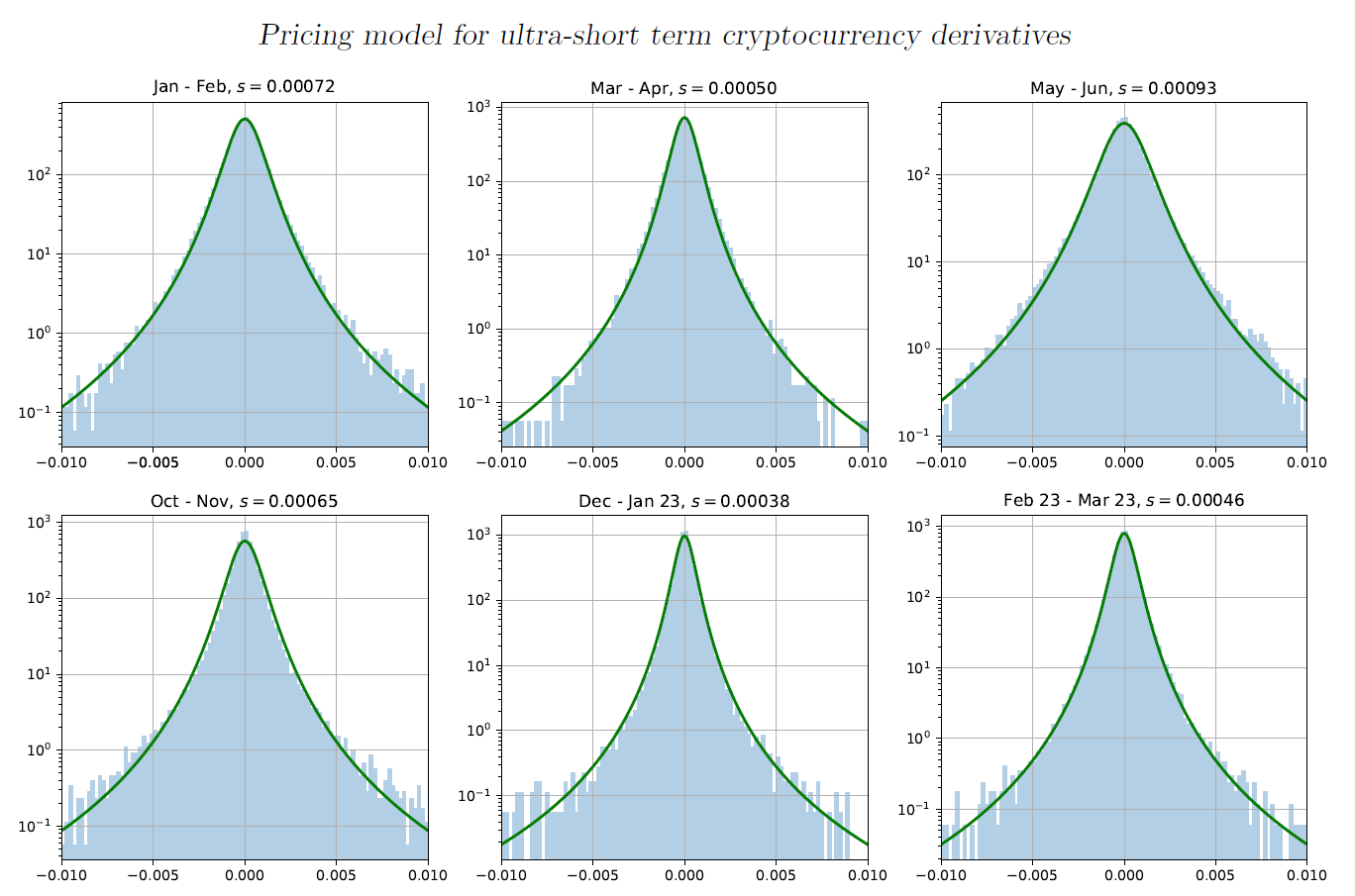
Continuing this analysis for other 2-month periods in our data set we can see in Fig. 3 that the shape of the distribution is always well represented by our model with dimensionality equal to 3, but the scale of the distribution changes with time. This is commonly referred to as heteroscedasticity. Such behaviour means that to use our model for derivatives pricing we need to establish the method of predicting the distribution scale (commonly referred to as volatility) for the upcoming period. But before that, we need to find out whether the model is suitable for price fluctuations over longer periods, in our case 30 to 90 minutes.

Fig. 3. Heteroscedastic behavior of price fluctiation distribution.

Analysis of historical ETH/USD price data at longer intervals

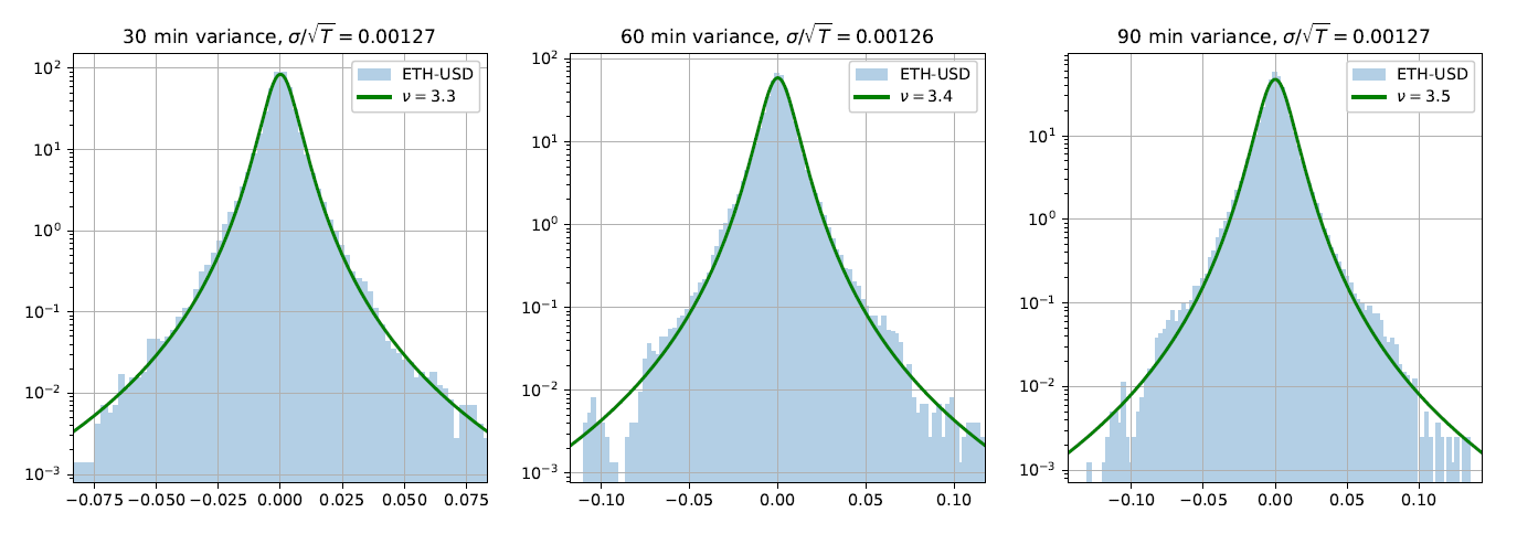
The comparison of the price fluctuation distribution over different periods is presented in Fig. 4. The charts show that our model can well represent distributions for periods from 30 to 90 minutes. The scale of the model is proportional to the square root of the period, while dimensionality gradually increases from 3.3 to 3.5. This means that we can use the same model for derivatives pricing in the range we are interested in.

Fig. 4. Distribution of price fluctuations over a longer period. The dimensionality parameter of the model increases with the increase of the period.

Volatility predictor model

As can be seen from the charts on Fig. 2-4 the shape of the price fluctuation distribution is well approximated by our model, so it would be very easy to price derivatives post factum. To offer a practically usable pricing method, we need to find a way to predict the distribution scale for the upcoming period. Prediction of volatility is a common concern for all derivate pricing models, so there is a large body of research on the subject (a good overview can be found in Filipovic & Khalilzade, 2021). In general, those methods fall into two categories: those that only use price history data and those that include fundamental economic factors. In our case maturity periods are so short that it does not make sense to try to take into account fundamental factors. One notable exception would be the situation when the timing of the fundamental event is known in advance. For example, the amount of rewards Bitcoin miners receive for each transaction block is set to halve at predetermined intervals. Such an event will likely be awaited by the majority of traders anticipating the change in the Bitcoin value and looking forward to trading in this opportunity. This increased trading activity is likely to suddenly increase volatility not only of Bitcoin but many other cryptocurrencies as well. Even common market events, such as the Federal Reserve's decision on the prime rate can have a ripple effect on cryptocurrency.

Such events and resulting changes in volatility cannot be predicted by any method based on historical data. Nevertheless, such events are pretty rare and for derivatives with ultra-short maturity periods, it is more practical to suspend trading in anticipation of major events than try to model them. For the rest of the time, we will use historical data for volatility prediction. We will aim to use the method with the smallest possible number of parameters. While the power and affordability of the algorithms based on neural networks/machine learning are very promising, we chose not to go this way for two reasons. Firstly, the results obtained via machine learning are not transparent. After training the model on a large set of data, we receive essentially a large number of coefficients of the chosen neural network. While there is some research on interpreting those matrices in subject matter terms, there is no generally accepted solution. Secondly, the number of parameters in modern ML models is huge and therefore there is a risk of overfitting the model.

Our approach is based on two pillars. The first is the use of robust metrics. The second is to build a predictor by combining metrics from the multiple receding periods (such as 30 min, 1 hour, 2 hours, 4 hours, 6 hours and 12 hours).

The use of robust metrics is preferable for the estimation of parameters of distributions with long tails, as metrics such as standard deviation can be easily skewed by outliers. We have chosen median absolute deviation (MAD) as a metric.

We found it necessary to combine the metrics calculated over multiple periods because short-period metrics, such as preceding 30 minutes, have a lot of variance in them that in most cases does not correspond to material changes in market conditions, but when such change does take place, they respond quickly to it. Metrics calculated over longer periods are more stable, but too slow to respond to the changes in market conditions. To obtain an estimate that is both reasonably stable and responsive, we use a linear combination of the estimates from multiple periods.

This can be compared to the composition of a square shape from sine waves of different periods, as illustrated in Fig.5.

Fig. 5. Illustration of the square shape composition from sine waves.

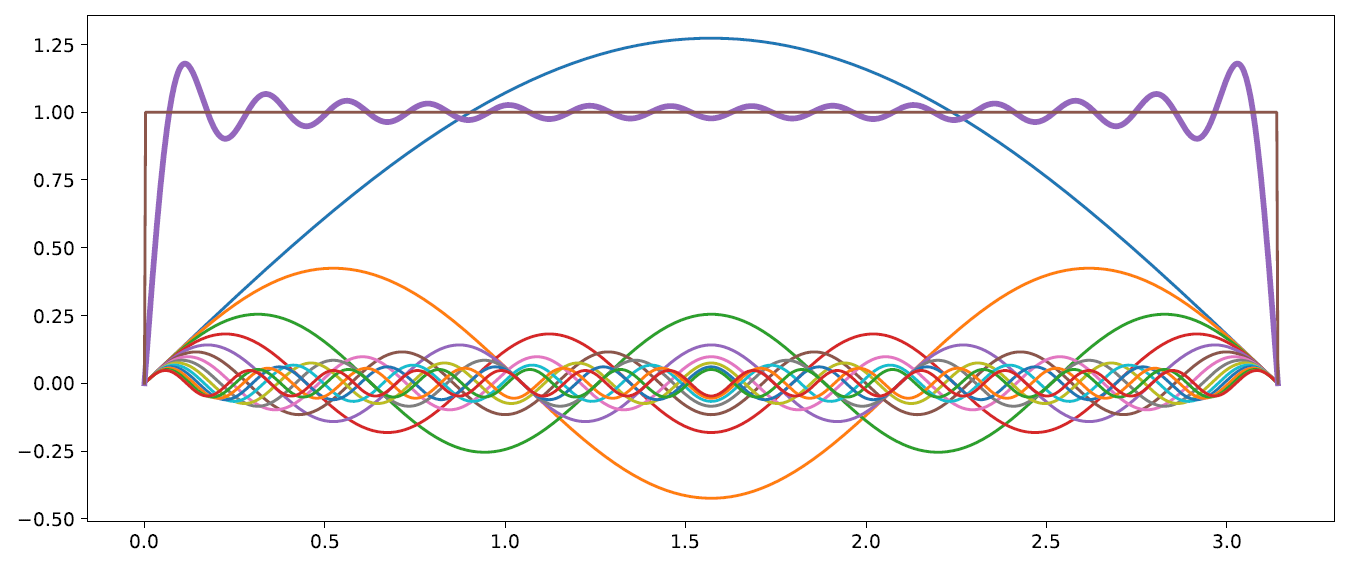
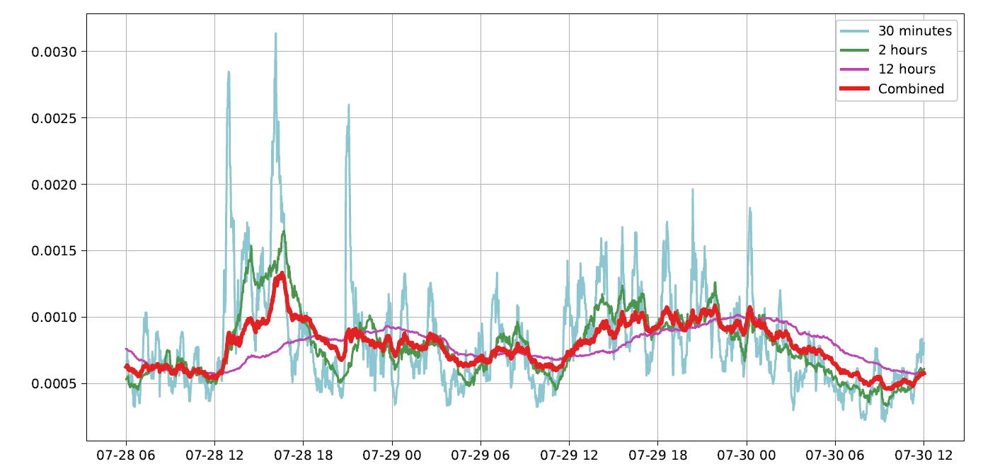
Similarly to how the square shape is approximated by the sum of sine waves, with the weight of those waves diminishing with the decrease in the period, we build our predictor by combining MAD estimates for periods from 12 hours down to 30 minutes. The weights of the estimates also diminish with the decrease in the period. The sample of the resulting predictor is shown in Fig 6. We can see that the 30-minute MAD estimate has many big spikes, most of which do not correspond to changes in volatility. On the other hand, the 12-hour estimate does not have big spikes but is not responding quickly enough to the increase in volatility that happened around noon on the 28th of July, 2022. If our pricing were based on a 12-hour estimate only, it would continue giving unreasonably low prices for several hours after the increase in volatility started.

Fig. 6. MAD volatility predictor example. The data covers the range from 6 a.m. on July 28 to noon on July 30, 2022.

Option pricing model for ultra-short periods

The options contract is a well-established trading instrument. It gives the buyer of the option the ability to obtain most of the yield in the underlying security without having to purchase it. Instead, the buyer is charged an amount that is much lower than the value of the security. For example, let’s assume that the current price of the ETH is 1,800 USD. The trader who believes that the value of the ETH is going to appreciate would consider buying a call option. The seller of the option would present an option chain, which is a set of strike prices and corresponding premiums for a specific maturity date. For example, the trader may buy the option with a strike price of $2,000 for $10. For this low premium, the buyer of the option obtains the right to buy the underlying security for $2,000. If the price of ETH reaches $2,100 by the time of maturity, the trader stands to earn $2,100 - $2,000 - $10 = $90 on this trade. The trader, of course, only profits when the price at maturity exceeds the strike price. The sellers of the option set strike prices in such a way that on average they stand to earn money for the risk they are taking.

The problem with ultra-short-term options is that well-established pricing models do not work. The traditional approach, developed by Black, Scholes, and Merton, is based on the assumption of random geometric walk, which implies that the distribution of price fluctuations $(r = log(p/p0))$ is normal. As we have established in the previous sections, for periods that we are interested in (30 to 90 minutes) this is not the case. To understand the problem, let’s have a look at the pricing problem from a statistical point of view. The cost of option $C$ for the strike price $K$, having the current price $S$, should be set in such a way that the profit for the seller of the option is equal to the expected value of the buyer’s return. The seller’s profit always equals $C$ and the buyer's return is the difference between the strike price $K$ and the maturity price $P(r) = Se^r$, when the maturity price is higher than the strike price (i.e. $r > log(K/S)$), and zero otherwise. To calculate EV we need to integrate the buyer’s return multiplied by probability density function $N(r)$ over all applicable $r$ values.

$$C = S (\int_{log(K/S)}^{\infty}e^rN(r)\,dr-K \int_{log(K/S)}^{\infty}N(r)\,dr$$

It can be shown that when $N(r)$ is a probability density function of a normal distribution, the equation (5.1) is equivalent to the Black-Scholes formula (assuming there is no known trend in the asset price and that the risk-free interest rate is zero, which is justified for ultra-short maturity periods). When the distribution $N(r)$ has tails that follow power law, the first integral in (5.1) is not going to converge, meaning that at any cost level $C$ the seller of the option will be losing money in the long run.

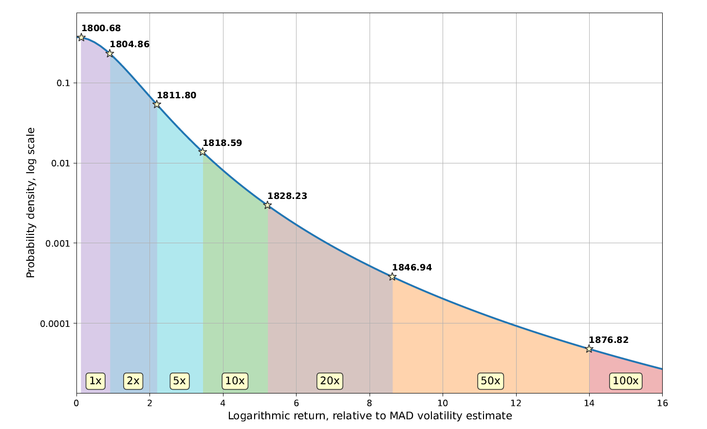
To overcome that difficulty, while preserving the similarity to the option, we introduce the following derivative instrument. Instead of a traditional option chain, the seller of the option should present the buyer with the price ladder, which is the list of prices and corresponding returns. The returns are relative to the size of the purchase. This concept is illustrated in Fig. 7. It assumes that the current price of ETH is $1,800 and that the buyer is interested in the call-type transaction (i.e. is expecting the price of ETH to go up). If the price of ETH reaches $1,812 at the time of maturity, the buyer will be paid 5 times the amount of purchase, if it reaches $1,830 - 20 times. If the price stays below $1,800.68, then the buyer does not get any returns.

Profit Ladder Multiplier	Probability	EV
0	0.547	0
1	0.24	0.24
2	0.16	0.32
5	0.036	0.18
10	0.012	0.12
20	0.004	0.08
50	0.0008	0.04
100	0.0002	0.02

The proposed derivative instrument shares similarities with a traditional American-style option. Traders have the opportunity to capitalize on asset (ETH) price movements by paying a relatively small amount up front.

Fig. 7. Profit ladder for ETH/USD call transaction.

The table shows the design of the instrument. The goal of the design was to keep the instrument interesting and engaging for traders while limiting the risk for the sellers. Almost half of all transactions (45.3%) result in a profit to the trader. At the same time, only 2% of the profit's EV is allocated to 100x profits, reducing the risk of the seller.

Testing and fine-tuning the option pricing model

To test the performance of the proposed instrument we have created a computer simulation in Python. The program uses 1-minute historical price data. For each minute it calculates the price ladder using data available before that moment. After that, it simulates one call and one put transaction, for a fixed amount. The results of all transactions are recorded and summarized for analysis.

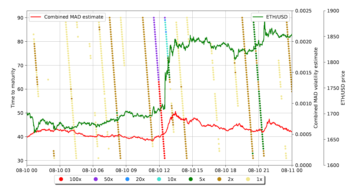
Figure 8 shows the subset of the simulation outcomes. We have selected the period that included significant price movement. Due to its size, all transactions starting from 64 minutes before the maturity time of 2 p.m. on the 10th of August resulted in maximum profits. The volatility estimator reflected the increase in volatility caused by this price movement fairly quickly, and transactions with maturity at 3 p.m. had considerably smaller returns.

Fig. 8. Sample result of trade simulation. Call option trade results, August 10 - 11.

The main characteristic we focus on is Return To Purchase (RTP), which is defined as the total of all profits divided by the total of all purchases. Note that we assume zero margin for the seller, which means that the measured RTT should be close to 100%.

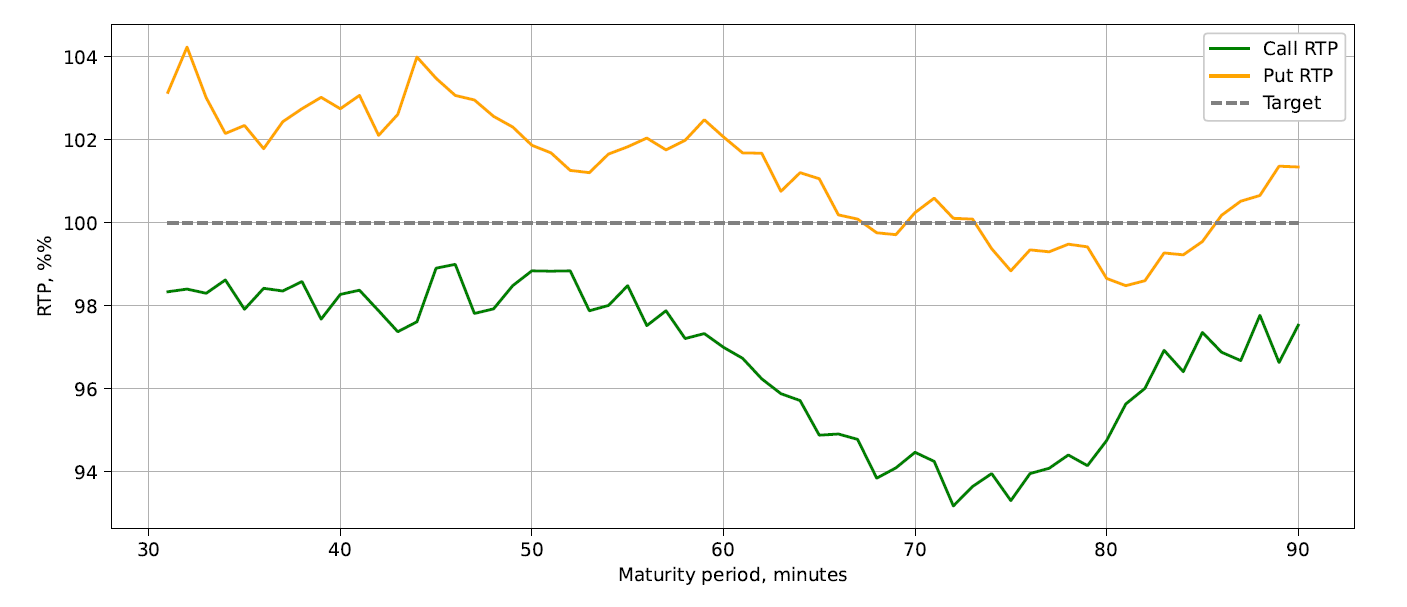
The initial results of the simulation on the 15-month testing period (Jan 1, 2022, to September 1, 2023) yielded reasonable overall results, as shown in Figure 9. At the same time, the breakdown of RTP by maturity time showed that it is not uniform, with transactions initiated 70-80 minutes to maturity having noticeably lower RTP (Figure 10).

Fig. 9. Monthly returns of simulated trading over testing period.

Fig. 10. Distribution of RTP over transaction maturity time.

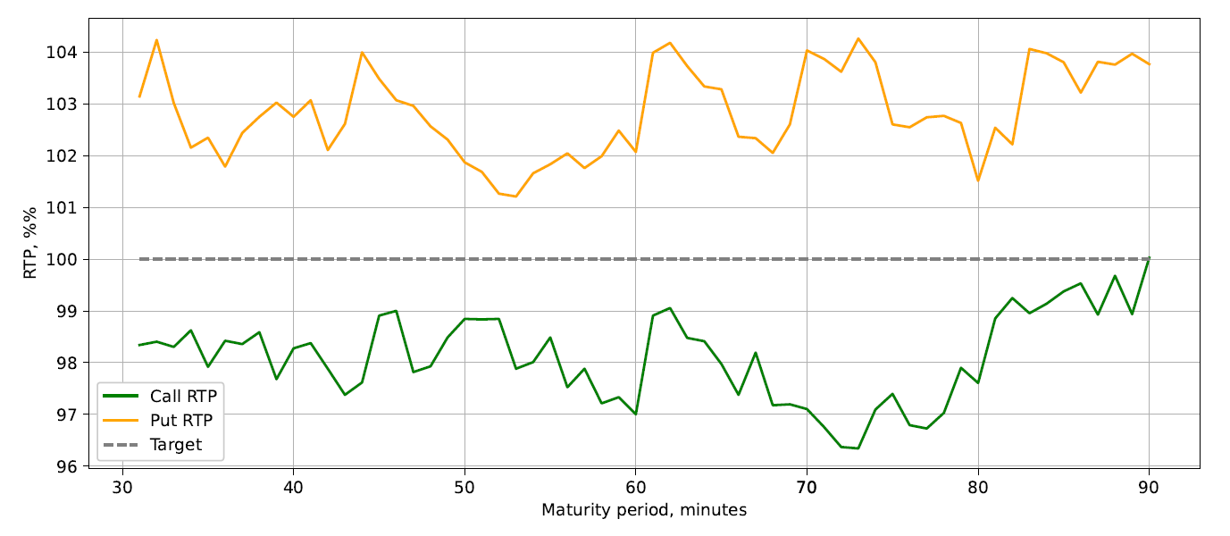
After reviewing the implementation of the simulation program, we made an assumption to simplify the calculations. The difference in dimensionality parameter of our model (from 3.3 to 3.5 depending on maturity time) was considered insignificant and a single value was used for all maturity times. Once that dependency was taken into account, the results have noticeably improved, as shown in Figure 11. While there are differences between the outcome of the call and put transactions, there is no discernible dependency of the RTP from the time to maturity. The reason for put transactions outperforming call transactions is that from time to time the price of the asset has a consistent trend up or down. As the model cannot predict the presence, duration or future scope of such trends, it is natural to expect that during periods of up-trend call transactions will have an advantage, and during periods of down-trend - put transactions.

Fig. 11. Distribution of RTP over transaction maturity time, with variable dimensionality parameter.

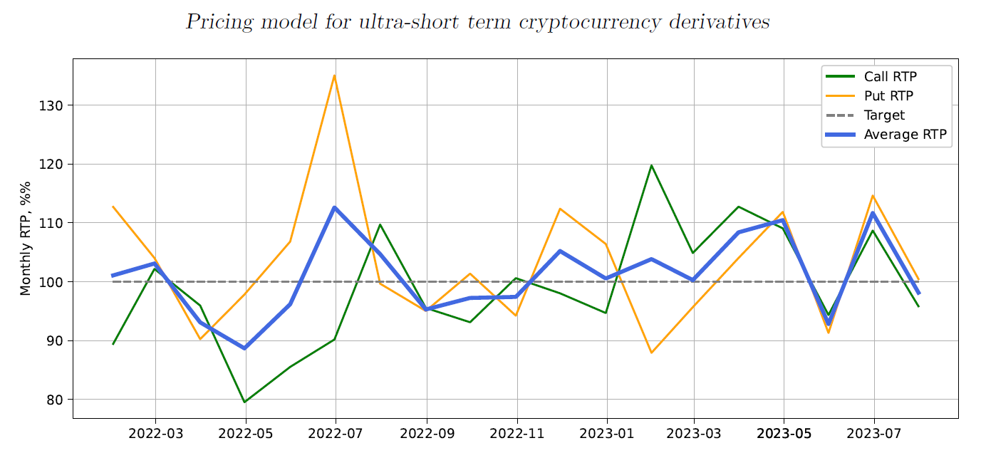
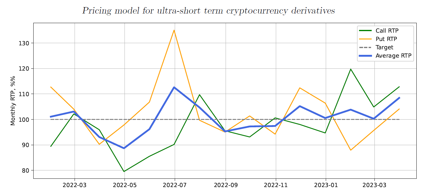
This difference in performance between put and call is more obvious in Figure 12, which shows the breakdown of RTP by month. As expected, most of the time the performance of put and call transactions deviates in opposite directions.

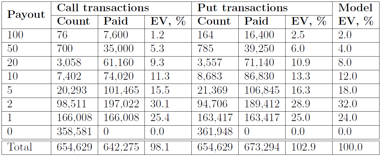
The following table summarizes all recorded transactions. It shows that our derivative instrument behaves very closely to expected values on pretty much any front. The overall RTP for the period is 98.1% for call transactions and 102.9% for put transactions, with a combined RTP of 100.5%, which is remarkably close to our target. The distribution of profits by profit value is also close to expected, even though higher profits do not have enough values to have good confidence intervals.

Fig. 12. Monthly returns of simulated trading, full correction.

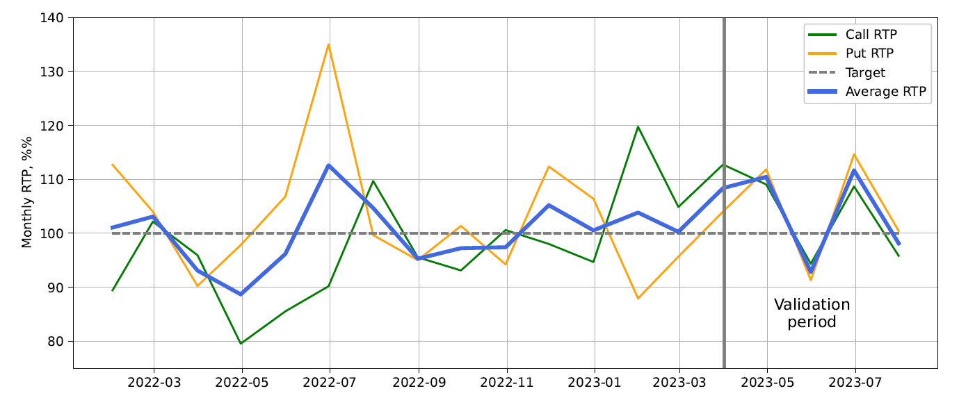
Let’s now see how the fully tuned model works on the out-of-band data, from April 1, 2023, to July 31, 2023. This is a harsh test, as the behaviour of the ETH/USD price (refer to Fig.1) is notably different from the period used for model development:

• The volatility during the validation period is several times lower than was observed during model development.

• The price of ETH is mostly moving “sideways”. During the training period, there was always either an up or down trend, but for the whole validation period, it stayed in a narrow channel.

Simulation result: CallRTP = 101.9%, PutRTP = 104.4%, or 103.15% on average. The breakdown by month is shown in Figure 13. The first thing that catches attention is that call and put performance is now very close and they deviate together from the expected RTP value. This should be expected, given that the price of ETH barely changed during that period, and there were no significant trends up or down. The overall RTP is almost 3% higher than what was observed during model development. While it could be the result of a lower number of trades during the validation period leading to higher variance, we will need to investigate whether there is any systemic factor at play. One avenue for further analysis is to explore how the volatility predictor works in a low-volatility environment.

Fig. 13. Monthly returns of simulated trading, including validation period.

Summary

To summarize, we have developed a pricing model tailored for short-term cryptocurrency options trading. The model consistently achieves higher accuracy and reduced premiums than the targeted ones and extends the trading period up to the remaining 30-minute cut-off mark. The model includes a range of customizable parameters for data sampling and volatility computations, allowing real-time adjustments to optimize performance in response to actual market dynamics.

References

[1] Benoit Mandelbrot, New Methods in Statistical Economics, Journal of Political Economy. 71, 1963, 421–440.

[2] D. Filipovic and A. Khalilzadeh, Machine Learning for Predicting Stock Return Volatility, Swiss Finance Institute. Research Paper Series N°21-95, 2021, 1–61.

[3] S. Maslov and M. Mills, Price Fluctuations from the Order Book Perspective - Empirical Facts and a Simple Model, Physica A: Statistical Mechanics and its Applications.